The Digitizing module of NeuLAND (R3B::Neuland::Digitizer) acts as an layer between the Geant4 generated R3BNeulandPoint and the real physical data R3BNeulandHit. The point data generated from the simulation engine contains the energy deposition of different particles. However, the physical hit data calculated through the calibration process don't distinguish the energy depositions among different particles. And the resulting energy deposition of the hit data normally represents total energy deposition of the event. There are other effects from both the scintillators and digitizing channels that could influence times, positions and energies of the final hit. the following sections include detailed information how the digitizing module helps to imitate the real physical processes and reduce the difference between the simulated data and the real data.

The technical programming details of this module are explained in the following document:

The Design principle of NeuLAND Digitizing module

General

The real data digitization of NeuLAND detector involves PMTS and multiple electronic modules, such as FQT, TAMEX-3, slow control units and the "back plates" which holds multiple FQT-TAMEX pairs and manage their communications to the data acquisition system. In this page, these processes are simplified into two different components: paddle and channel. The name "paddle" comes from the old prototype of NeuLAND, in which the scintillators looks like paddles with different values of height and width. the "channel" component incorporates everything between the scintillator output and the storage of the binary data. On the other hand, the Digitizing module needs to provide the data of R3BNeulandHit, which is similar to the step from the calibration process (R3B::Neuland::Cal2HitTask). In the future, the digitizing module may use the same task from the calibration to generate hit level data. For now, it is using its own process to construct the resulting hit level data (see the picture below).

Figure 1: NeuLAND Digitizing Dataflow

Paddle component

The paddle component in the digitizing module is related to the class R3B::Digitizing::Neuland::Paddle.

Paddle related parameters

The component contains following parameters:

Parameter	Default value	Unit	Explanation
`attenuation`	0.008	1/cm	Light attenuation factor
`effective_speed`	8.	cm/ns	Effective speed of light in the scintillator
`time_offset`	0.	ns	Local time offset parameter
`time_sync`	0.	ns	Gloabl time sync parameter

They are used in three different physical processes:

attenuation is used for calculating the reduction of the light intensity when traveling through the scintillator. The light intensity received by the PMTs on the both ends, $I_{l/r}$, can be described as:

$$ \begin{align} \label{eq:atten_1} I_{l} &= I_0 \cdot e^{-\alpha(L/2 + x )}\\ \label{eq:atten_2} I_{r} &= I_0 \cdot e^{-\alpha(L/2 - x )} \end{align} $$

with:
- $x$: The distance of the energy deposition to the center of the bar (right direction is the positive direction).
- $I_0$: The initial energy deposition value.
- $L$: The length of the scintillation bar
- $\alpha$: The attenuation factor
Effective_speed represents the traveling speed of the scintillation photons inside the scintillator. The value of the effective speed of light isn't entirely same as the speed of light of in the material, but also accounts for the light reflection during the traveling.
Time related parameters like time_offset and time_sync come from the time delays introduced by the different length of the cables connecting to each PMT. The signal time of left/right PMT, $t_{l/r}$, can be calculated as

$$ \begin{align} t_l &= t + (L/2 - x)/c_e + D_l\\ t_r &= t + (L/2 + x)/c_e + D_r \end{align} $$

with:
- $x$: The distance of the energy deposition to the center of the bar.
- $t$: The initial time of the energy deposition.
- $c_e$: Effective speed of light.
- $L$: The length of the scintillation bar.
- $D_{l/r}$: The time delays of the cables connecting to the left/right PMT.
By redefining $D_{l/r}$ in terms of global time synchronization factor ( $t_\text{sync}$) and local time offset parameter ( $t_\text{offset}$) with:

$$ \begin{align} t_\text{offset} &= D_r - D_l\\ t_\text{sync} &= \left(D_r + D_l\right)/2 \end{align} $$

The signal times of the left and right PMTs can be expressed as:

$$ \begin{align} \label{eq:delay_1} t_l = t + (L/2 + x)/c_e - t_\text{offset}/2 + t_\text{sync}\\ \label{eq:delay_2} t_r = t + (L/2 - x)/c_e + t_\text{offset}/2 + t_\text{sync} \end{align} $$

Construction of paddle signals

As can be seen in Fig. 1, the first action of the paddle class is to construct signals (R3B::Digitizing::PaddleSignal) from point data (R3BNeulandPoint). The data representing the paddle signal contains three variables: time, energy deposition and the distance to the center point of the paddle. It should be noticed that except the time value, the position and energy values from the point data cannot be directly used for the paddle signal data. Position values from the point data (see R3BNeulandPoint::GetPosition()) represent global coordinates of the energy depositions and should be converted to local distances to the paddle center with the function R3BNeulandGeoPar::ConvertToLocalCoordinates(). On the other hand, the energy of the point data (obtained by R3BNeulandPoint::GetLightYield()) is in the unit of GeV while the energy of paddle signal is in the unit of MeV. For the next time, the constructed paddle signal is used to calculate the channel signals for the two PMTs on the both ends.

Construction of channel signals

Construction of the channel signals is based on two physical effects:

Light attenuation, involving parameters in equations $\ref{eq:atten_1}$ and $\ref{eq:atten_2}$: light attenuation factor $\alpha$
Time delays from cables, involving parameters in equations $\ref{eq:delay_1}$ and $\ref{eq:delay_2}$: effective speed of light $c_e$, global time synchronization $t_\text{sync}$ and local time offset $t_\text{offset}$

Each paddle signal generates two channel signals (R3B::Digitizing::ChannelSignal) in total, one for the left side and the other for the right side. The only difference between the constructions of the two channel signals is the opposite sign of the distance to the center point. If the energy deposition happens on the right side of the center point, the distance value is positive and vice versa for the other side.

Construction of paddle hits

A paddle hit (R3B::Digitizing::PaddleHit) is constructed by two channel hits. If each channel only has one channel hit, the energy of the constructed paddle hit can be obtained by multiply equation $\ref{eq:atten_1}$ with equation $\ref{eq:atten_2}$, which yields:

$$ \begin{equation} I_0 = \sqrt{I_l \cdot I_r} \cdot e^{\alpha L / 2} \end{equation} $$

The position of the paddle hit can be calculated by subtracting equation $\ref{eq:delay_1}$ from equation $\ref{eq:delay_2}$:

$$ \begin{equation} \label{eq:position} x = \frac{c_e}{2} (t_l - t_r + t_\text{offset}) \end{equation} $$

where as the time can be obtained from the summation of the two equations:

$$ \begin{equation} t = \frac{t_l + t_r}{2} - \frac{L}{2c_e} -t_\text{sync} \end{equation} $$

Channel hit matching

Depending on the channel configurations (see Fig. 2 below), especially on the signal pileup strategy, multiple channel hits could be generated in a channel in some rare events. In such case, a matching algorithm could be performed so that only the two channel hits from the same energy deposition are used for the paddle hit construction.

Figure 2: Multiplicity of signals/hits per event using different methods

The criterion for recognizing two channel hits caused by the same energy deposition is derived from the division between equation $\ref{eq:atten_2}$ and $\ref{eq:atten_1}$, with $x$ replaced by equation $\ref{eq:position}$:

$$ \begin{equation} I_r / I_l = e^{\alpha\cdot c_e (t_l - t_r + t_\text{offset})} \end{equation} $$

by putting all variable on the same side, one gets the criterion equation:

$$ \begin{align} I_l / I_r \cdot e^{\alpha c_e (t_l - t_r + t_\text{offset})} - 1 &\rightarrow 0\qquad&\text{if}\quad t_l - t_r + t_\text{offset} > 0 \\ I_r / I_l \cdot e^{\alpha c_e (t_r - t_l - t_\text{offset})} - 1 &\rightarrow 0\qquad&\text{if}\quad t_l - t_r + t_\text{offset} < 0 \end{align} $$

The right match can be found if it has the smallest value from the left side. The reason of the condition on $t_l - t_r + t_\text{offset}$ is to make sure the wrong match results in a significantly larger value than the right match. If the exponent value $t_l - t_r + t_\text{offset}$ is a negative value, the exponential value can only be between $0 \sim 1$, which makes it way harder to distinguish the right match from the wrong one.

Channel component

The channel component of NeuLAND is implemented in two different classes:

The JSON option tasks.NeulandDigitizer.channel can be specified to choose which of the two classes is used. It's highly recommended to use tamex channel as it implements the functionalities of the latest digitizer, TAMEX-3. For the following sections, details about the tamex channel class are explained.

Tamex related parameters

Parameters can be found in the class R3B::Digitizing::Neuland::Tamex::Params and can be specified by the JSON field tasks.NeulandDigitizer.par in the JSON configuration file.

Parameter	Default value	Unit	Explanation
`energy_gain`	15.0	ns/MeV	Energy gain paramter
`pedestal`	14.0	ns	Pedestal (energy baseline) parameter
`energy_res_rel`	0.05	MeV	Relative energy resolution
`time_res`	0.15	ns	Time resolution
`pmt_thresh`	1.	MeV	PMT threshold
`saturation_coefficient`	0.012		Saturation coefficent of the PMT
`max_time`	1000.	ns	Maximal time
`min_time`	1.	ns	Minimal time
`min_energy`	0.067	MeV	Minimal energy
`pileup_time_window`	1000.	ns	The time window for the pileup
`pileup_distance`	100.	ns	Distance value for the pileup

some further information:

The relation between the energy and ToT (time-over-threshold) of the signal can be described with two parameters: energy_gain and pedestal using the equation:

$$ \begin{equation} \label{eq:gain} t_\text{ToT} = G \cdot E + t_0 \end{equation} $$

where $t_\text{ToT}$ is the time over threshold, $G$ the gain factor, $E$ the energy value and $t_0$ the pedestal value.
The PMT saturation factor saturation_coefficient is to depict the non-linearity between the ToT and its input energy when the energy value is very large. Thus, before applying equation $\ref{eq:gain}$, a saturated energy is calculated instead:

$$ \begin{equation} \label{eq:sat_energy} E_\text{sat} = \frac{E}{1 + \lambda E} \end{equation} $$
Smearing parameters time_res and energy_res_rel randomize the time and energy values of channel hits (see section Generation of channel hits below).
Pileup related parameters pileup_time_window and pileup_distance will only be used if the corresponding pileup method is chosen (see section Generation of Cal signals below).

Generation of Cal signals

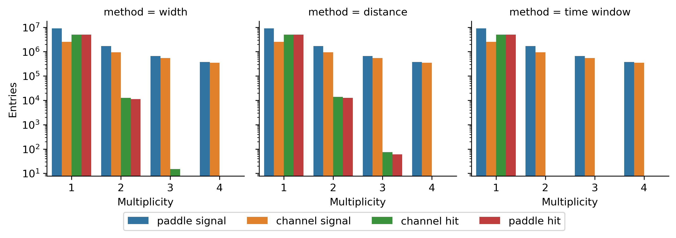
A cal signal is typically constructed by multiple channel signals, as can be seen in Fig. 2 where the multiplicity of the channel signals is substantially reduced before producing channel hits. Each channel signal is usually corresponding to the energy deposition from different particles. But in the real experiment, those signals from different particles are piled up as one single signal. In this Tamex channel module, there are three different ways (see Tamex::PeakPileUpStrategy) to achieve the pileup of particle-induced channel signals: width, distance and time_window.

The procedures to convert channel signals (R3B::Digitizing::ChannelSignal) to the cal signals (R3B::Digitizing::ChannelCalSignal) can be described in order with:

A new channel signal is inputted by calling the private virtual function Tamex::Channel::add_signal. The time of the channel signal is checked whether it follows the condition below:

$$ \begin{equation} t_\text{min} < t < t_\text{max} \end{equation} $$

where $t_\text{min}$ and $t_\text{max}$ can be specified by the parameters max_time and min_time. If the condition is not met, the signal will be discarded.
If the condition is met, the signal will be converted to a PMT signal in the type Neuland::Tamex::PMTPeak. The time of the PMT signal is the same as the time value from the channel signal. The calculation of the height of the PMT signal is calculated from the saturation effect (equation $\ref{eq:sat_energy}$) where the height is $E$ and the parameter saturation_coefficient is $\lambda$. The converted PMT signal is then pushed to a vector for further processing.
Once the public method Digitizing::Engine::Construct() is called in the digitizer task, the vector of PMT signals start to be converted to a vector of FQT peaks (Neuland::Tamex::FQTPeak) in order:
1. The vector of PMT signals is sorted with increasing time values.
2. Each adjacent PMT signals in the vector are piled up if they follow the pileup criterion (see section Pileup strategies below for more details).
3. Check the height of each piled up PMT signal and remove those whose height is below the threshold value specified by the parameter pmt_thresh.
4. After the pileup and filtering with the threshold, each PMT signal is then converted to the FQT signal. Again, the time and the energy of the FQT signal can be directly obtained from the time and the height of the PMT signal respectively. The FQT time_over_thresh value is calculated by using the FQT energy value as E in equation $\ref{eq:gain}$.
5. The converted FQT peaks are then again piled up depending on different pile strategies.
The time-over-threshold and the leading edge time of the Cal signal are simply the time_over_thresh and leading_edge_time value of the FQT peak.

The reason why there is two additional data structures (PMT peaks and FQT peaks) during the conversion from channel signals to Cal signals is based on the different natures of signal pileup in the real experiment. If the leading edges of the two PMT signals are very closed, the energy of the resulting piled-up signal is simply the summation of the two. However, same principle cannot be applied for the two reshaped signals (FQT signals) when they are partially overlapped with each other. Thus, It requires different pileup strategies other than simple summation. The available pileup strategies for the reshaped signals (FQT signals) can be seen in section Pileup strategies below.

Another subtlety should be noted during the conversion from the energy value to the time-over-threshold value. In the calibration algorithm (see R3BNeulandCal2Hit::Exec()), the energy value is calculated with:

$$ \begin{equation} \label{eq:energy} E = \max \{ t_\text{ToT} - t_0, 1 \} / G \end{equation} $$

where $t_\text{ToT}$, $G$ and $t_0$ is the time-over-threshold, PMT gain and pedestal value respectively. Thus the inverse of the relation is undefined for time-over-threshold values smaller than 1 ns. To eliminate this undefined behavior, the conversion from $t_\text{ToT}$ to the energy isn't exactly the same as equation $\ref{eq:gain}$, but with an additional condition:

$$ \begin{aligned} t_\text{ToT} &= G \cdot E + t_0 \qquad&\text{if}\quad E > E_\text{min} \\ t_\text{ToT} &= G \cdot E \cdot (t_0 + 1) \qquad&\text{if}\quad E < E_\text{min} \end{aligned} $$

with the minimum energy threshold $E_\text{min} = 1 / G$ to make sure the conversion is still a continuous function.

Pileup strategies

The pileup between different signals is the main mechanism to reduce the large multiplicities from the simulator. In the Tamex channel, there are two signals, namely PMT and FQT signals, that are piled up:

The pileup of the PMT signals is straightforward and simple as it's just the summation of their amplitudes (heights) if the time difference between the two signals are smaller than 15 ns. This is based on the fact that if two protons deposit their energy at the same time, the corresponding energy value of the pileup signal should be equal to the summation.
The pileup of the reshaped signals (FQT signals) is uncertain and requires further investigation. Currently there are three strategies specified by the user:
- time_window: The FQT signals are first sorted with increasing time. All the signals whose time values are withn $[t_\text{min}, \ \ t_\text{min} + t_\text{window}]$ are added up where $t_\text{min}$ is the time of the earliest signal and $t_\text{window}$ is specified by the pileup_time_window parameter. The addition of the two signals are done by summing up their energy values and the time-over-threshold of the piled-up signal is recalculated from the summed energy value. The time of the piled-up signal is $t_\text{min}$.
- distance: The "distance" pileup strategy also begins with the sorting with increasing time. Then the time difference between the leading edges of each consecutive signals is checked. If the time difference is less than pileup_distance parameter, the two signal will be piled up in the same way as in time_window method.
- width: This strategy utilizes the width (time difference between the leading edge and trailing edge) of each FQT signal. Again, signals are first sorted with the increasing time value. Then each two consecutive signals are checked whether they are overlapped with each other by identifying whether the trailing edge time of the former signal is larger than the leading edge time of the latter signal. If they overlap with each other, the two signals will be piled up in such way that the new piled-up signal has the leading edge time equal to the one from the former signal and the trailing edge time equal to the one of the latter signal. The time-over-threshold is then calculated based on the time difference of the leading and trailing edges. The energy value of the new signal is calculated from its time-over-threshold value using equation $\ref{eq:energy}$.

The Cal signal data, which only contains time-over-threshold value, leading edge time and the channel side cannot be directly used for the calibration algorithm. However, if one tries to verify the calibration algorithms via the simulated cal level data, the Cal signal data can be converted to the cal level data (Neuland::BarCalData) through a conversion task (Neuland::SimCal2Cal).

Generation of channel hits

Channel hits of the Tamex channel module are constructed from the piled-up FQT signals without reducing the multiplicity during the process (see Tamex::Channel::CreateHit()). It goes through the following processes:

The energy and time values from the FQT peaks are smeared with a Gaussian distribution whose $\sigma$ value is specified by the parameters energy_res_rel and time_res respectively. For example, the output energy value can also be expressed with the equation below:

$$ \begin{equation} \label{eq:randEnergy} E_\text{smear} \sim \mathcal{N}(E, \sigma^2) \end{equation} $$

where the output smeared energy value is sampled from the Gaussian distribution. Similar equation can also be applied to the time value.
Convert the smeared energy value back to the unsaturated value with the equation:

$$ \begin{equation} E = \frac{E_\text{sat}}{ 1 - E_\text{sat} \cdot \lambda} \end{equation} $$

which is the inverse of equation $\ref{eq:sat_energy}$.

Table of Contents